Inference with pyLFI

Example usage of the pyLFI for parameter identification.

import matplotlib.pyplot as plt
import numpy as np
import pylfi
import scipy.stats as stats

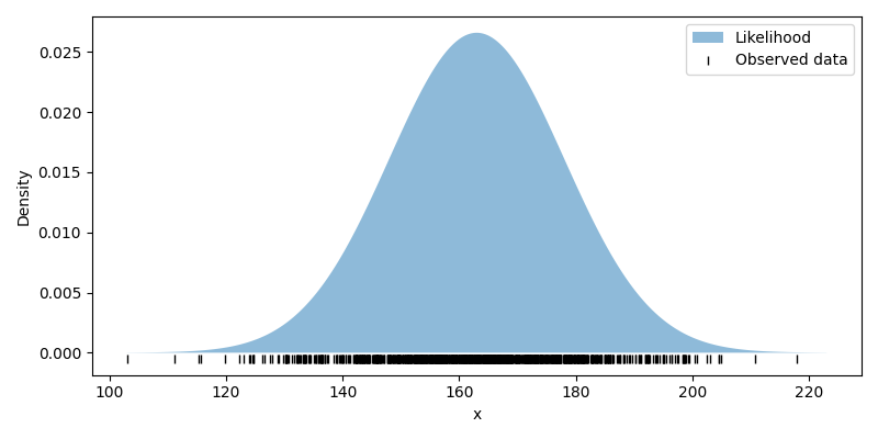
In the following, we demonstrate pyLFI on a toy example. We will infer the model parameters of a univariate Gaussian distribution: the mean \(\mu\) and standard deviation \(\sigma\). In this toy example, the likelihood is \(p (y_\mathrm{obs} \mid \mu, \sigma) = \mathrm{N(\mu=163, \sigma=15)}\), and the observed data are sampled from the likelihood:

mu_true = 163
sigma_true = 15
likelihood = stats.norm(loc=mu_true, scale=sigma_true)
obs_data = likelihood.rvs(size=1000)

x = np.linspace(103, 223, 1000)
likelihood_pdf = likelihood.pdf(x)
fig, ax = plt.subplots(figsize=(8, 4), tight_layout=True)
pylfi.utils.densityplot(x, likelihood_pdf, ax=ax, label='Likelihood')
pylfi.utils.rugplot(obs_data, pos=-0.0005, ax=ax, label='Observed data')
ax.set(xlabel='x', ylabel='Density')
ax.legend()

Out:

<matplotlib.legend.Legend object at 0x7f130bd62ca0>

We assume that the likelihood is unknown, and formulate a model to describe the observed data. The model needs to be implemented as a Python callable, i.e., a function or a __call__ method in a class, that is parametrized by the unknown model parameters we aim to infer, here \(\mu\) and \(\sigma\):

def simulator(mu, sigma, size=1000):
    y_sim = stats.norm(loc=mu, scale=sigma).rvs(size=size)
    return y_sim

Next, we need to reduce the raw data into low-dimensional summary statistics. The summary statistics calculator also needs to be implemented as a Python callable. The function must return the summary statistics as a Python list or numpy.ndarray. Here, we take the mean and standard deviation to be summary statistics of the data (these are actually sufficient summary statistics):

def stat_calc(y):
    sum_stats = [numpy.mean(y), numpy.std(y)]
    return sum_stats

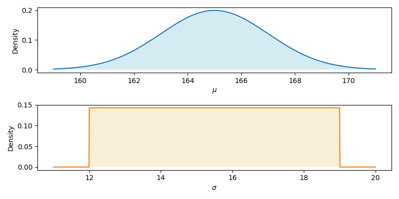
We then place priors over the unknown model parameters using the Prior class. In the present example, we define the priors:

mu_prior = pylfi.Prior('norm',
                       loc=165,
                       scale=2,
                       name='mu',
                       tex=r'$\mu$'
                       )

sigma_prior = pylfi.Prior('uniform',
                          loc=12,
                          scale=7,
                          name='sigma',
                          tex=r'$\sigma$'
                          )

priors = [mu_prior, sigma_prior]

fig, axes = plt.subplots(nrows=2, figsize=(8, 4), tight_layout=True)
x = np.linspace(159, 171, 1000)
mu_prior.plot_prior(x, ax=axes[0])
x = np.linspace(11, 20, 1000)
sigma_prior.plot_prior(x, color='C1', facecolor='wheat', ax=axes[1])

previous

Using the pyLFI Prior class

next

API Reference